Optical Components of the Eye
Reflections From the Eye
Linear Systems Methods
Shift-Invariant Linear Transformations
- Shift-Invariant Systems: Definition
- Shift-Invariant Systems: Properties
The Optical Quality of the Eye
- The Linespread Function
- The Modulation Transfer Function
Lenses, Diffraction and Aberrations

Image Formation

The cornea and lens are at the interface between the physical world of light and the neural encoding of the visual pathways. The cornea and lens bring light into focus at the light sensitive receptors in our retina and initiate a series of visual events that result in our visual experience.

The initial encoding of light at the retina is but the first in a series of visual transformations: The stimulus incident at the cornea is transformed into an image at the retina. The retinal image is transformed into a neural response by the light sensitive elements of the eye, the photoreceptors. The photoreceptor responses are transformed to a neural response on the optic nerve. The optic nerve representation is transformed into a cortical representation, and so forth. We can describe most of our understanding of these transformations, and thus most of our understanding of the early encoding of light by the visual pathways by using linear systems theory. Because all of our visual experience is limited by the image formation within our eye, we begin by describing this transformation of the light signal and we will use this analysis as an introduction to linear methods.

Optical Components of the Eye

Figure 2.1: The imaging components of the eye. The cornea and lens focus the image onto the retina. Light enters through the pupil which is bordered by the iris. The fovea is a region of the retina that is specialized for high visual acuity and color perception. The retinal output fibers leave at a point in the retina called the blindspot. The bundle of output fibers is called the optic nerve.

Figure 2.1 contains an overview of the imaging components of the eye. Light from a source arrives at the cornea and is focused by the cornea and lens onto the photoreceptors, a collection of light sensitive neurons. The photoreceptors are part of a thin layer of neural tissue, called the retina. The photoreceptor signals are communicated through the several layers of retinal neurons to the neurons whose output fibers makes up the optic nerve. The optic nerve fibers exit through a hole in the retina called the optic disk. The optical imaging of light incident at the cornea into an image at the retinal photoreceptors is the first visual transformation. Since all of our visual experiences are influenced by this transformation, we begin the study of vision by analyzing the properties of image formation.

When we study transformations, we must specify their inputs and outputs. As an example, we will consider how simple one-dimensional intensity patterns displayed on a video display monitor are imaged onto the retina (Figure 2.2a). In this case the input is the light signal incident at the cornea. One-dimensional patterns have a constant intensity along the, say, horizontal dimension and varies along the perpendicular (vertical) dimension. We will call the pattern of light intensity we measure at the monitor screen the monitor image. We can measure the intensity of the one-dimensional image by placing a light-sensitive device called a photodetector at different positions on the screen. The vertical graph in Figure 2.2b shows a measurement of the intensity of the monitor image at all screen locations.

The output of the optical transformation is the image formed at the retina. When the input image is one-dimensional, the retinal image will be one-dimensional, too. Hence, we can represent it using a curve as in Figure 2.2c. We will discuss the optical components of the visual system in more detail later in this chapter, but from simply looking at a picture of the eye in Figure 2.1 we can see that the monitor image passes through a lot of biological material before arriving at the retina. Because the optics of the eye are not perfect, the retinal image is not an exact copy of the monitor image: The retinal image is a blurred copy of the input image.

The image in Figure 2.2b shows one example of an infinite array of possible input images. Since there is no hope of measuring the response to every possible input, to characterize optical blurring completely we must build a model that specifies how any input image is transformed into a retinal image. We will use linear systems methods to develop a method of predicting the retinal image from any input image.

Figure 2.2: Retinal image formation illustrated with a single-line input image. (a) A one-dimensional monitor image consists of a set of lines at different intensities. The image is brought to focus on the retina by the cornea and lens. (b) We can represent the intensity of a one-dimensional image using a simple graph that shows the light as a function of horizontal screen position. Only a single value is plotted since the one- dimensional image is constant along the vertical dimension. (c) The retinal image is a blurred version of the one-dimensional input image. The retinal image is also one-dimensional and is also represented by a single curve.

Reflections From the Eye

To study the optics of a human eye you will need an experimental eye, so you might invite a friend to dinner. In addition, you will need a light source, such as a candle, as a stimulus to present to your friend’s eye. If you look directly into your friend’s eye, you will see a mysterious darkness that has beguiled poets and befuddled visual scientists. The reason for the darkness can be understood by considering the problem of ophthalmoscope design illustrated in Figure 2.3a.

Figure 2.3: Principles of the ophthalmoscope. An ophthalmoscope is used to see an image reflected from the interior of the eye. (a) When we look directly into the eye, we cast a shadow making it impossible to see light reflected from the interior of the eye. (b) The ophthalmoscope permits us to see light reflected from the interior of the eye. Helmholtz invented the first ophthalmoscope. (After Cornsweet, 1970).

If the light source is behind you, so that your head is between the light source and the eye you are studying, then your head will cast a shadow that interferes with the light from the point source arriving at your friend’s eye. As a result, when you look in to measure the retinal image you see nothing beyond what is in your heart. If you move to the side of the light path, the image at the back of your friend’s eye will be reflected towards the light source, following a reversible path. Since you are now on the side, out of the path of the light source, no light will be sent towards your eye.

Figure 2.4: A modified opthalmoscope measures the human retinal image. Light from a bright source passes through a slit and into the eye. A fraction of the light is reflected from the retina and is imaged. The intensity of the reflected light is measured at dif- ferent spatial positions by varying the location of the analyzing slit. (After Campbell and Gubisch, 1967).

Flamant (1955) first measured the retinal image using a modified ophthalmoscope. She modified the instrument by placing a light sensitive recording, a photodetector, at the position normally reserved for the ophthalmologist’s eye. In this way, she measured the intensity pattern of the light reflected from the back of the observer’s eye. Campbell and Gubisch (1967) used Flamant’s method to build their apparatus, which is sketched in Figure 2.4. Campbell and Gubisch measured the reflection of a single bright line, that served the input stimulus in their experiment. As shown in the Figure, a beam-splitter placed between the input light and the observer’s eye divides the input stimulus into two parts. The beam-splitter causes some of the light to be turned away from the observer and lost; this stray light is absorbed by a light baffle. The rest of the light continues toward the observer. When the light travels in this direction, the beam-splitter is an annoyance, serving only to lose some of the light; it will accomplish its function on the return trip.

Figure 2.5: The retina contains the light sensitive photoreceptors where light is fo- cussed. This cross-section of a monkey retina outside the fovea shows there are sev- eral layers of neurons in the optical path between the lens and the photoreceptors. As we will see later, in the central fovea these neurons are displaced to leaving a clear optical path from the lens to the photoreceptors (Source: Boycott and Dowling, 1969).

The light that enters the observer’s eye is brought to a good focus on the retina by a lens. A small fraction of the light incident on the retina is reflected and passes – a second time – through the optics of the eye. On the return path of the light, the beam-splitter now plays its functional role. The reflected image would normally return to a focus at the light source. But the beam-splitter divides the returning beam so that a portion of it is brought to focus in a measurement plane to one side of the apparatus. Using a very fine slit in the measurement plane, with a photodetector behind it, Campbell and Gubisch measured the reflected light and used the measurements of the reflected light to infer the shape of the image on the retinal surface.

What part of the eye reflects the image? In Figure 2.5 we see a cross-section of the peripheral retina. In normal vision, the image is focused on the retina at the level of the photoreceptors. The light measured by Campbell and Gubisch probably contains components from several different planes at the back of the eye. Thus, their measurements probably underestimate the quality of the image at the level of the photoreceptors.

Figure 2.6 shows several examples of Campbell and Gubisch’s measurements of the light reflected from the eye when the observer is looking at a very fine line. The different curves show measurements for different pupil sizes. When the pupil was wide open (top, 6.6mm diameter) the reflected light is blurred more strongly than when the pupil is closed (middle, 2.0mm). Notice that the measurements made with a large pupil opening are less noisy; when the pupil is wide open more light passes into the eye and more light is reflected, improving the quality of the measurements.

The light measured in Figure 2.6 passed through the optical elements of the eye twice, while the retinal image passes through the optics only once. It follows that the spread in these curves is wider than the spread we would observe had we measured at the retina. How can we use these doublepass measurements to estimate the blur at the retina? To solve this problem, we must understand the general features of their experiment. It is time for some theory.

Figure 2.6: Experimental measurements of light that has been reflected from a human eye looking at a fine line. The reflected light has been blurred by double passage through the optics of the eye. (Source: Campbell and Gubisch, 1966).

Linear Systems Methods

A good theoretical account of a transformation, such as the mapping from monitor image to retinal image, should have two important features. First, the theoretical account should suggest to us which measurements we should make to characterize the transformation fully. Second, the theoretical account should tell us how to use these measurements to predict the retinal image distribution for all other monitor images.

In this section we will develop a set of general tools, referred to as linear systems methods. These tools will permit us to solve the problem of estimating the optical transformation from the monitor to the retinal image. The tools are sufficiently general, however, that we will be able to use them repeatedly throughout this book.

There is no single theory that applies to all measurement situations. But, linear systems theory does apply to many important experiments. Best of all, we have a simple experimental test that permits us to decide whether linear systems theory is appropriate to our measurements. To see whether linear systems theory is appropriate, we must check to see that our data satisfy the two properties of homogeneity and superposition.

Homogeneity

Figure 2,7: Homogeneity -The principle of homogeneity illustrated. An input stimulus and corresponding retinal image are shown in each part of the figure. The three input stimuli are the same except for a scale factor. Homogeneity is satisfied when the corresponding retinal images are scaled by the same factor. Part (a) shows an input image at unit intensity, while (b) and (c) show the image scaled by 0.5 and 2.0 respectively

A test of homogeneityis illustrated in Figure 2.7 The left-hand panels show a series of monitor images, and the right-hand panels show the corresponding measurements of reflected light ¹. Suppose we represent the intensities of the lines in the one-dimensional monitor image using the vector $\pixvec$ (upper left) and we represent the retinal image measurements by the vector $\resvec$ . Now, suppose we scale the input signal by a factor $a$ , so that the new input is $a \pixvec$ . We say that the system satisfies homogeneity if the output signal is also scaled by the same factor of $a$ , and thus the new output is $a \resvec$ . For example, if we halve the input intensity, then the reflected light measured at their photodetector should be one-half the intensity (middle panel). If we double the light intensity, the response should double (bottom panel). Campbell and Gubisch’s measurements of light reflected from the human eye satisfy homogeneity.

¹ We will use vectors and matrices in our calculations to eliminate burdensome notation. Matrices will be denoted by boldface, upper case Roman letters, $\bf M$ . Column vectors will be denoted using lower case boldface Roman letters, ${\bf v}$ . The transpose operation will be denoted by a superscript T, ${\bf v}^T$ . Scalar values will be in normal typeface, and they will usually be denoted using Roman characters ( $a$ ) except when tradition demands the use of Greek symbols ( $\alpha$ ). The $i^{th}$ entry of a vector, ${\bf v}$ , is a scalar and will be denoted as $v_i$ . The $i^{th}$ column of a matrix, $\bf M$ , is a vector that we denote as ${\bf m}_i$ . The scalar entry in the $i^{th}$ row and $j^{th}$ column of the matrix ${\bf M}$ will be denoted $m_{ij}$ .

Superposition

Figure 2.8: Superposition. The principle of superposition} illustrated. Each of the three parts of the picture shows an input stimulus and the corresponding retinal image. The stimulus in part (a) is a single-line image and in part (b) the stimulus is a second line displaced from the first. The stimulus in part (c) is the sum of the first two lines. Superposition holds if the retinal image in part (c) is the sum of the retinal images in parts (a) and (b).

Superposition, used as both an experimental procedure and a theoretical tool, is probably the single most important idea in this book. You will see it again and again in many forms. We describe it here for the first time.

Suppose we measure the response to two different input stimuli. For example, suppose we find that input pattern $\pixvec$ (top left) generates the response $\resvec$ (top right), and input pattern $\pixvec '$ (middle left) generates response $\resvec '$ (middle right). Now we measure the response to a new input stimulus equal to the sum of $\pixvec$ and $\pixvec '$ . If the response to the new stimulus is the sum of the responses measured singly, $\resvec + \resvec '$ , then the system is a linear system. By measuring the responses stimuli individually and then the response to the sum of the stimuli, we test superposition. When the responses to sum of the stimuli equals the sum of the individual responses, then we say the system satisfies superposition. Campbell and Gubisch’s measurements of light reflected from the eye satisfy this principle.

We can summarize homogeneity and superposition succinctly using two equations. Write the linear optical transformation that maps the input image to the light intensity at each of the receptors as:

(1) $\begin{equation*} {\mbox{$r_{#1}$}}= L ({\mbox {$\bf p$} }) ~~~ \end{equation*}$

Homogeneity and superposition are defined by the pair of equations:

(2) $\begin{eqnarray*} L ( a \mbox {$\bf p$} ) = & a L ( \mbox {$\bf p$} ) & (~Homogeneity~) \\ L ( \mbox {$\bf p$} + \mbox {$\bf p$} ' ) = & L ( \mbox {$\bf p$} ) + L ( \mbox {$\bf p$}' ) & (~Superposition~) \end{eqnarray*}$

Implications of Homogeneity and Superposition

Application of homogeneity and superposition

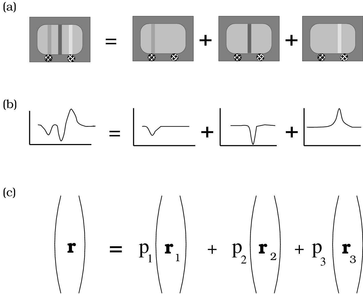
Figure 2.9: (a) A one-dimensional monitor image is the weighted sum of a set of lines. An example of a one-dimensional image is shown on the left and the individual monitor lines comprising the monitor image are shown separately on the right. (b) Each line in the component monitor image contributes to the retinal image. The retinal images created by the individual lines are shown below the individual monitors. The sum of the retinal images is shown on the left. (c) The retinal image generated by …

Figure 2.9 illustrates how we will use linear systems methods to characterize the relationship between the input signal from a monitor, light reflected from the eye (we analyze a one-dimensional monitor image to simplify the notation. The principles remain the same, but the notation becomes cumbersome when we consider two-dimensional images.). First, we make an initial set of measurements of the light reflected from the eye for each single-line monitor image, with the line set to unit intensity. If we know the images from single-line images, and we know the system is linear, then we can calculate the light reflected from the eye from any monitor image: Any one-dimensional image is the sum of a collection of lines.

Consider an arbitrary one-dimensional image, as illustrated at the top of Figure 2.9. We can conceive of this image as the sum of a set of single-line monitor images, each at its own intensity, $\pixveci{i}$ . We have measured the reflected light from each single-line image alone, call this $\resvec_i$ for the $i^{th}$ line. By homogeneity it follows that the reflected light from $i^{th}$ line will be a scaled version of this response, namely $\pixveci{i} \resvec_i$ .. Next, we combine the light reflected from the single-line images. By superposition, we know that the light reflected from the original monitor image, $\resvec$ , is the sum of the light reflected from the single-line images,

(3) $\begin{equation*} \resvec = \sum_i^{N} \pixveci{i} \resvec_i . \end{equation*}$

The above equation defines a transformation that maps the input stimulus, $\pixvec$ , into the measurement, $\resvec$ . Because of the properties of homogeneity and superposition, the transformation is the weighted sum of a fixed collection of vectors: When the monitor image varies, only the weights in the formula, $\pixveci{i}$ , vary but the vectors $\resvec_i$ , the reflections from single-line stimuli, remain the same. Hence, the reflected light will always be the weighted sum of these reflections.

To represent the weighted sum of a set of vectors, we use the mathematical notation of matrix multiplication. As shown in Figure 2.8, multiplying a matrix times a vector computes the weighted sum of the matrix columns; the entries of the vector define the weights. Matrix multiplication and linear systems methods are closely linked. In fact, the set of all possible matrices define the set of all possible linear transformations of the input vectors.

Figure 2.10: Matrix multiplication – is a convenient notation for linear systems methods. For example, the weighted sum of a set of vectors, as in part (c) of Figure 2.7, can be represented using matrix multiplication. The matrix product equals the sum of the columns of … weighted by the entries of …. When the matrix describes the responses of a linear system, we call it a system matrix.

Matrix multiplication has a shorthand notation to replace the explicit sum of vectors in Equation 3. In the example here, we define a matrix, $\Resmat$ , whose columns are the responses to individual monitor lines at unit intensity, $\resvec_i$ . The matrix $\Resmat$ is called the system matrix. Matrix multiplication of the input vector, $\pixvec$ , times the system matrix $\Resmat$ , transforms the input vector into the output vector. Matrix multiplication is written using the notation

(4) $\begin{equation*} \resvec = \Resmat \pixvec . \end{equation*}$

Matrix multiplication follows naturally from the properties of homogeneity and superposition. Hence, if a system satisfies homogeneity and superposition, we can describe the system response by creating a system matrix that transforms the input to the output.

A numerical example of a system matrix.

sys = [ 0.1 0 0 ; 0.2 0.1 0 ; 0.5 0.2 0.2; 0.3 0.5 0.5 ; 0 0.1 0.3 ; 0 0 0 ]; p = [0.5 1 0.2]; sys* p’

Let’s use a specific numerical example to illustrate the principle of matrix multiplication. Suppose we measure a monitor that displays only three lines. We can describe the monitor image using a column vector with three entries, $\pixvec = (p_1, p_2, p_3)^T$ .

The lines of unit intensity are $(1,0,0)^T$ , $(0,1,0)^T$ and $(0,0,1)^T$ . We measure the response to these input vectors to build the system matrix. Suppose the measurements for these three lines are $(0.1,0.2,0.5,0.3,0,0)^T$ , $(0,0.1,0.2,0.5,0.1,0)^T$ , and $(0,0,0.2,0.5,0.3,0)^T$ respectively.

We place these responses into the columns of the system matrix:

(5) $\begin{equation*} \Resmat = \left ( \begin{array}{ccc} 0.1 & 0 & 0 \\ 0.2 & 0.1 & 0 \\ 0.5 & 0.2 & 0.2 \\ 0.3 & 0.5 & 0.5 \\ 0 & 0.1 & 0.3 \\ 0 & 0 & 0 \end{array} \right ) \end{equation*}$

We can predict the response to any monitor image using the system matrix. For example, if the monitor image is $\pixvec = (0.5,1.0,.2)^T$ we multiply the input vector and the system matrix to obtain the response, on the left side of Equation 6.

(6) $\begin{equation*} \left ( \begin{array}{c} 0.05 \\ 0.20 \\ 0.49 \\ 0.75 \\ 0.16 \\ 0 \end{array} \right ) = \left ( \begin{array}{ccc} 0.1 & 0 & 0 \\ 0.2 & 0.1 & 0 \\ 0.5 & 0.2 & 0.2 \\ 0.3 & 0.5 & 0.5 \\ 0 & 0.1 & 0.3 \\ 0 & 0 & 0 \end{array} \right ) \left ( \begin{array}{c} 0.5 \\ 1.0 \\ 0.2 \end{array} \right ) \end{equation*}$

Why Linear Methods are Useful

Linear systems methods are a good starting point for answering an essential scientific question: How can we generalize from the results of measurements using a few stimuli to predict the results we will obtain when we measure using novel stimuli? Linear systems methods tell us to examine homogeneity and superposition. If these empirical properties hold in our experiment, then we will be able to measure responses to a few stimuli and predict responses to many other stimuli.

This is very important advice. Quantitative scientific theories are attempts to characterize and then explain systems with many possible input stimuli. Linear systems methods tell us how to organize experiments to characterize our system: measure the responses to a few individual stimuli, and then measure the responses to mixtures of these stimuli. If superposition holds, then we can obtain a good characterization of the system we are studying. If superposition fails, your work will not be wasted since you will need to explain the results of superposition experiments to obtain a complete characterization of the measurements.

To explain a system, we need to understand the general organizational principles concerning the system parts and how the system works in relationship to other systems. Achieving such an explanation is a creative act that goes beyond simple characterization of the input and output relationships. But, any explanation must begin with a good characterization of the processing the system performs.

Shift-Invariant Linear Transformations

Shift-Invariant Systems: Definition

Since homogeneity and superposition are well satisfied by Campbell and Gubisch’s experimental data, we can predict the result of any input stimulus by measuring the system matrix that describes the mapping from the input signal to the measurements at the photodetector. But the experimental data are measurements of light that has passed through the optical elements of the eye twice, and we want to know the transformation when we pass through the optics once. To correct for the effects of double passage, we will take advantage of a special property of optics of the eye, shift-invariance. Shift-invariant linear systems are an important class of linear systems, and they have several properties that make them simpler than general linear systems. The following section briefly describes these properties and how we take advantage of them. The mathematics underlying these properties is not hard; I sketch proofs of these properties in the Appendix.

Suppose we start to measure the system matrix for the Campbell and Gubisch experiment by measuring responses to different lines near the center of the monitor. Because the quality of the optics of our eye is fairly uniform near the fovea, we will find that our measurements, and by implication the retinal images, are nearly the same for all single-line monitor images. The only way they will differ is that as the position of the input translates, the position of the output will translate by a corresponding amount. The shape of the output, however, will not change. An example of two measurements we might find when we measure using two lines on the monitor is illustrated in the top two rows of Figure 2.8. As we shift the input line, the measured output shifts. This shift is a good feature for a lens to have, because as an object’s position changes, the recorded image should remain the same (except for a shift). When we shift the input and the form of the output is invariant, we call the system shift-invariant.

Shift-Invariant Systems: Properties

We can define the system matrix of a shift-invariant system from the response to a single stimulus. Ordinarily, we need to build the system matrix by combining the responses to many individual lines. The system matrix of a linear shift-invariant system is simple to estimate since these responses are all the same except for a shift. Hence, if we measure a single column of the matrix, we can fill in the rest of the matrix. For a shift-invariant system, there is only one response to a line. This response is called the linespread of the system. We can use the linespread function to fill in the entire system matrix.

The response to a harmonic function at frequency $f$ is a harmonic function at the same frequency. Sinusoids and cosinusoids are called harmonics or harmonic functions. When the input to shift-invariant system is a harmonic at frequency $f$ , the output will be a harmonic at the same frequency. The output may be scaled in amplitude and shifted in position, but it still will be a harmonic at the input frequency.

For example, when the input stimulus is defined at $N$ points and at these points its values are sinusoidal, $\SfNi$ . Then, the response of a shift-invariant system will be a scaled and shifted sinusoid, $s_f \sin ( \pfiN + \phi_f )$ . There is some uncertainty concerning the output because there two unknown values, the scale factor, $s_f$ , and phase shift, $\phi_f$ . But, for each sinusoidal input we know a lot about the output; the output will be a sinusoid of the same frequency as the input.

We can express this same result another useful way. Expanding the sinusoidal output using the summation rule we have

(7) $\begin{equation*} s_f \sin (\pfiN + \phi_f ) = a_f \cos (\pfiN) + b_f \sin (\pfiN) . \end{equation*}$

where

(8) $\begin{eqnarray*} a_f &=& s_f \sin ( \phi_f) \nonumber \\ b_f &=& s_f \cos ( \phi_f ). \end{eqnarray*}$

In other words, when the input is a sinusoid at frequency $f$ , the output is the weighted sum of a sinusoid and a cosinusoid, both at the same frequency as the input. In this representation, the two unknown values are the weights of the sinusoid and the cosinusoid.

For many optical systems, such as the human eye, the relationship between harmonic inputs and the output is even simpler. When the input is a harmonic function at frequency $f$ , the output is a scaled copy of the function and there is no shift in spatial phase. For example, when the input is $\SfNi$ the output will be $s_f \SfNi$ , and only the scale factor, which depends on frequency, is unknown.

The Optical Quality of the Eye

We are now ready to correct the measurements for the effects of double passage through the optics of the eye. To make the method easy to understand, we will analyze how to do the correction by first making the assumption that the optics introduce no phase shift into the retinal image; this means, for example, that a cosinusoidal stimulus creates a cosinusoidal retinal image, scaled in amplitude. It is not necessary to assume that there is no phase shift but the assumption is reasonable and the main principles of the analysis are easier to see if we assume there is no phase shift.

Figure 2.11: Sinusoids and Double Passage (a) The amplitude, A, of an input cosinusoid stimulus is scaled by a factor, s, after passing through even-symmetric shift-invariant symmetric optics as shown in part (b). (c) Passage through the optics a second time scales the amplitude again, resulting in a signal with amplitude s^2 A.

To understand how to correct for double passage, consider a hypothetical alternative experiment Campbell and Gubisch might have done Figure 2.11. Suppose Campbell and Gubisch had used input stimuli equal to cosinusoids at various spatial frequencies, $f$ . Because the optics are shift-invariant and there is no frequency-dependent phase shift, the retinal image of a cosinusoid at frequency $f$ is a cosinusoid scaled by a factor $s_f$ . The retinal image passes back through the optics and is scaled again, so that the measurement would be a cosinusoid scaled by the factor ${s_f}^2$ . Hence, had Campbell and Gubisch used a cosinusoidal input stimulus, we could deduce the retinal image from the measured image easily: The retinal image would be a cosinusoid with an amplitude equal to the square root of the amplitude of the measurement.

Campbell and Gubisch used a single line, not a set of cosinusoidal stimuli. But, we can still apply the basic idea of the hypothetical experiment to their measurements. Their input stimulus, defined over $N$ locations, is

(9) $\begin{equation*} \pixveci{i} = \left\{ \begin{array}{ll} 1 & \mbox{if $i=0$} \\ 0 & \mbox{if $1 \leq i < N$} \end{array} \right. \end{equation*}$

As I describe in the appendix, we can express the stimulus as the weighted sum of harmonic functions by using the discrete Fourier series. The representation of a single line is equal to the sum of cosinusoidal functions

(10) $\begin{equation*} \pixvechati{i} = 0.5 + \sum_{f=1}^{f=N-1} \cos( 2 \pi f {i/N})~~. \end{equation*}$

Because the system is shift-invariant, the retinal image of each cosinusoid was a scaled cosinusoid, say with scale factor $s_f$ . The retinal image was scaled again during the second pass through the optics, to form the cosinusoidal term they measured².

² Be bothered by the fact that the discrete Fourier series approximation is an infinite set of pulses,rather than a single line. To understand why, consult the Appendix.

Using the discrete Fourier series, we also can express the measurement as the sum of cosinusoidal functions,

(11) $\begin{equation*} \mbox{Measurement} = 0.5 + \sum_{f=1}^{f=N-1} (s_f)^2 \cos( 2 \pi f {i/N}). \end{equation*}$

We know the values of ${s_f}^2$ , since this was Campbell and Gubisch’s measurement. The image of the line at the retina, then, must have been

(12) $\begin{equation*} \lspreadi{i} = 0.5 + \sum_{f=1}^{f=N-1} s_f \cos( 2 \pi f {i/N}). \end{equation*}$

Figure 2.12: The linespread function of the human eye: The solid line in each panel is a measurement of the linespread. The dotted lines are the diffraction-limited linespread for a pupil of that diameter. (Diffraction is explained later in the text). The different panels show measurements for a variety of pupil diameters (From Campbell and Gubisch, 1967).

The values $\lspreadi{i}$ define the linespread function of the eye’s optics. We can correct for the double passage and estimate the linespread because the system is linear and shift-invariant.

As you read further about experimental and computational methods in vision science, remember that there is nothing inherently important about sinusoids as visual stimuli; we must not confuse the stimulus with the system or with the theory we use to analyze the system. When the system is a shift-invariant linear system, sinusoids can be helpful in simplifying our calculations and reasoning, as we have just seen. The sinusoidal stimuli are important only insofar as they help us to measure or clarify the properties of the system. And if the system is not shift-invariant, the sinusoids may not be important at all.

The Linespread Function

Figure 2.12 contains Campbell and Gubisch’s estimates of the linespread functions of the eye. Notice that as the pupil size increases, the width of the linespread function increases which indicates that the focus is worse for larger pupil sizes. As the pupil size increases, light reaches the retina through larger and larger sections of the lens. As the area of the lens affecting the passage of light increases, the amount of blurring increases.

The measured linespread functions, $\lspreadi{i}$ , along with our belief that we are studying a shift-invariant linear system, permit us to predict the retinal image for any one-dimensional input image. To calculate these predictions, it is convenient to have a function that describes the linespread of the human eye. G. Westheimer (1986) suggested the following formula to describe the measured linespread function of the human eye, when in good focus, and when the pupil diameter is near 3mm.

(13) $\begin{equation*} \lspreadi{i} = 0.47 e^{ - 3.3 i ^ {2} } + 0.53 e ^ { -0.93 | i | } \end{equation*}$

where the variable $i$ refers to position on the retina specified in terms of minutes of visual angle. A graph of this linespread function is shown in Figure 2.13.

Figure 2.13: Westheimer’s Linespread Function. Analytic approximation of the human linespread function for an eye with a 3.0mm diameter pupil (Westheimer, 1986).

We can use Westheimer’s linespread function to predict the retinal image of any one-dimensional input stimulus ³. Some examples of the predicted retinal image are shown in Figure 2.13. Because the optics blurs the image, even the light from a very fine line is spread across several photoreceptors. We will discuss the relationship between the optical defocus and the positions of the photoreceptors in Chapter 3.

³ Westheimer’s linespread function is for an average observer under one set of viewing conditions. As the pupil changes size and as observer’s age, the linespread function can vary. Consult IJspeert et al. (1993) and Williams et al. (1995) for alternatives to Westheimer’s formula.

Figure 2.14: Retinal Images. Examples of the effect of optical blurring. (a) Images of a line, edge and a bar pattern. (b) The estimated retinal image of the images after blurring by Westheimer’s linespread function. The spacing of the photoreceptors in the retina is shown by the stylized arrows

The Modulation Transfer Function

In correcting for double passage, we thought about the measurements in two separate ways. Since our main objective was to derive the linespread function, a function of spatial position, we spent most of our time thinking of the measurements in terms of light intensity as a function of spatial position. When we corrected for double passage through the optics, however, we also considered a hypothetical experiment in which the stimuli were harmonic functions (cosinusoids). To perform this calculation, we found that it was easier to correct for double passage by thinking of the stimuli as the sum of harmonic functions, rather than as a function of spatial position.

Figure 2.15: Modulation transfer function measurements of the optical quality of the lens made using visual interferometry (Williams et al., 1995; described in Chapter 3). The data are compared with the predictions from the linespread suggested by Westheimer (1984) and a curve fit through the data by Williams et al. (1995).

These two ways of looking at the system, in terms of spatial functions or sums of harmonic functions, are equivalent to one another. To see this, notice that we can use the linespread function to derive the retinal image to any input image. Hence, we can use the linespread to compute the scale factors of the harmonic functions. Conversely, we already saw that by measuring how the system responds to the harmonic functions, we can derive the linespread function. It is convenient to be able to reason about system performance in both ways.

The optical transfer function defines the system’s complete response to harmonic functions. The optical transfer function is a complex-valued function of spatial frequency. The complex values code both the scale factor and the phase shift the system induces in each harmonic function.

When the linespread function of the eye is an even-symmetric function, there is no phase shift of the harmonic functions. In this case, we can describe the system completely using a real valued function, the modulation transfer function. This function defines the scale factors applied to each spatial frequency. The data points in Figure 2.15 show measurements of the modulation transfer function of the human eye. These data points were measured using a method called visual interferometry that is described in Chapter 3. Along with the data points in Figure 2.15, I have plotted the predicted modulation transfer function using Westheimer’s linespread function and a curve fit to the data by Williams et al. (1995). The curve derived by Westheimer (1986) using completely different data sets differs from the measurements by Williams et al. (1995) by no more than about twenty percent. This should tell you something about the relative precision of these descriptions of the optical quality of the lens.

The linespread function and the modulation transfer function offer us two different ways to think about the optical quality of the lines. The linespread function in Figure 2.15, describes defocus as the spread of light from a fine slit across the photoreceptors: the light is spread across three to five photoreceptors. The modulation transfer function in Figure 2.15 describes defocus as an amplitude reduction of harmonic stimuli: beyond 12 cycles per degree the amplitude is reduced by more than a factor of two.

Lenses, Diffraction and Aberrations

Lenses and Accommodation

What prevents the optics of our eye from focusing the image perfectly? To answer this question we should consider why a lens is useful in bringing objects to focus at all.

Figure 2.16: Snell’s law. The solid lines indicate surface normals and the dashed lines indicate the light ray. (a) When a light ray passes from one medium to another, the ray can be refracted so that the angle of incidence (phi) does not equal the angle of refraction (phi ‘). Instead, the angle of refraction depends on the refractive indices of the new media (n and n’) a relationship called Snell’s law that is defined in Equation :snell (after Jenkins and White figures 1H page 15 and 2H page 30.) (b) A prism causes two refractions of the light ray and can reverse the ray’s direction from upward to downward. (c) A lens combines the effect of many prisms in order to converge the rays diverging from a point source. (After Jenkins and White figure 1F, page 12.).

As a ray of light is reflected from an object, it will travel along along a straight line until it reaches a new material boundary. At that point, the ray may be either absorbed by the new medium, reflected, or refracted. The latter two possibilities are illustrated in part (a) of Figure 2.16. We call the angle between the incident ray of light and the perpendicular to the surface the angle of incidence. The angle between the reflected ray and the perpendicular to the surface is called the angle of reflection, and it equals the angle of incidence. Of course, reflected light is not useful for image formation at all.

The useful rays for imaging must pass from the first medium into the second. As they pass from between the two media, the ray’s direction is refracted. The angle between the refracted ray and the perpendicular to the surface is called the angle of refraction.

The relationship between the angle of incidence and the angle of refraction was first discovered by a Dutch astronomer and mathematician, Willebrord Snell in 1621. He observed that when $\phi$ is the angle of incidence, and $\phi '$ is the angle of refraction, then

(14) $\begin{equation*} \frac{ \sin \phi } { \sin \phi ' } = \frac{\nu '}{\nu } \end{equation*}$

The terms $\nu '$ and $\nu$ in Equation 14 are the refractive indices of the two media. The refractive index of an optical medium is the ratio of the speed of light in a vacuum to the speed of light in the optical medium. The refractive index of glass is $1.520$ , for water the refractive index is $1.333$ and for air it is nearly $1.000$ . The refractive index of the human cornea is $1.376$ is quite similar to water, which is the main content of our eyes.

Now, consider the consequence of applying Snell’s law twice in a row as light passes into and then out of a prism, as illustrated in part (b) of Figure 2.16. We can draw the path of the ray as it enters the prism using Snell’s law. The symmetry of the prism and the reversibility of the light path makes it easy to draw the exit path. Passage through the prism bends the ray’s path downward. The prism causes the light to deviate significantly from a straight path; the amount of the deviation depends upon the angle of incidence and the angle between the two sides of the prism.

We can build a lens by smoothly combining many infintesimally small prisms to form a convex lens, as illustrated in part (c) of Figure 2.16. In constructing such a lens, any deviations from the smooth shape, or imperfections in the material used to build the lens, will cause the individual rays to be brought to focus at slightly different points in the image plane. These small deviations of shape or materials are a source of the imperfections in the image.

Objects at different depths are focused at different distances behind the lens. The lensmaker’s equation relates the distance between the source and the lens with the distance between the image and the lens. The lensmaker’s equation relating these two distances depends on focal length of the lens. Call the distance from the center of the lens to the source $d_s$ , the distance to the image $d_i$ , and the focal length of the lens, $f$ . Then the lensmaker’s equation is

(15) $\begin{equation*} \frac{1}{{d_s}} + \frac{1}{{d_i}} = \frac{1}{ f} . \end{equation*}$

From this equation, notice that we can measure the focal length of a convex thin lens by using it to image a very distant object. In that case, the term $1/{d_s}$ is zero so that the image distance is equal to the focal length. When I first moved to California, I spent a lot of time measuring the focal length of the lenses in my laboratory by going outside and imaging the sun on a piece of paper behind the lens; the sun was a convenient source at optical infinity. It had been a less reliable source for me in my previous home.

Figure 2.17: Depth of Field in the Human Eye. Image distance is shown as a function of source distance. The bar on the vertical axis shows the distance of the retina from the lens center. A lens power of 60 diopters brings distant objects into focus, but not nearby objects; to bring nearby objects into focus the power of the lens must increase. The depth of field, namely the distance over which objects will continue to be in reasonable focus, can be estimated from the slope of the curve.

The optical power of a lens is a measure of how strongly the lens bends the incoming rays. Since a short focal length lens bends the incident ray more than a long focal length lens, the optical power is the inversely related to focal length. The optical power is defined as the reciprocal of the focal length measured in meters and is specified in units of diopters. When we view far away objects, the distance from the middle of the cornea and the flexible lens to the retina is 0.017m. Hence, the optical power of the human eye is $1/0.017 = 58.8$ , or roughly 60 diopters.

From the optical power of the eye ( $1/f$ ) and the lensmaker’s equation, we can calculate the image distance of a source at distance. For example, the top curve in Figure 2.17 shows the relationship between image distance $(d_i)$ and source distance $(d_s)$ for a 60 diopter lens. Sources beyond 1.0m are imaged at essentially the same distance behind the optics. Sources closer than 1.0m are imaged at a longer distance, so that the retinal image is blurred.

To bring nearby sources into focus on the retina, muscles attached to the lens change its shape and thus change the power of the lens. The bottom two curves in Figure 2.17 illustrate that sources closer than 1.0m can be focused onto the retina by increasing the power of the lens. The process of adjusting the focal length of the lens is called accommodation. You can see the effect of accommodation by first focusing on your finger placed near your noise and noticing that objects in the distance appear blurred. Then, while leaving your finger in place, focus on the distant objects. You will notice that your finger now appears blurred.

Pinhole Optics and Diffraction

The only way to remove lens imperfections completely is to remove the lens. It is possible to focus images without any lens at all by using pinholeoptics, as illustrated in Figure 2.18.

Figure 2.18: Pinhole Optics. Using ray-tracing, we see that only a small pencil of rays passes through a pinhole. (a) If we widen the pinhole, light from the source spread across the image, making it blurry. (b) If we narrow the pinhole, only a small amount of light is let in. The image is sharp; the sharpness is limited by diffraction.

A pinhole serves as a useful focusing element because only the rays passing within a narrow angle are used to form the image. As the pinhole is made smaller, the angular deviation is reduced. Reducing the size of the pinhole serves to reduce the amount of blur due to the deviation amongst the rays. Another advantage of using pinhole optics is that no matter how distant the source point is from the pinhole, the source is rendered in sharp focus. Since the focusing is due to selecting out a thin pencil of rays, the distance of the point from the pinhole is irrelevant and accommodation is unnecessary.

But the pinhole design has two disadvantages. First, as the pinhole aperture is reduced, less and less of the light emitted from the source is used to form the image. The reduction of signal has many disadvantages for sensitivity and acuity.

A second fundamental limit to the pinhole design is a physical phenomenon. When light passes through a small aperture, or near the edge of an aperture, the rays do not travel in a single straight line. Instead, the light from a single ray is scattered into many directions and produces a blurry image. The dispersion of light rays that pass by an edge or narrow aperture is called diffraction. Diffraction scatters the rays coming from a small source across the retinal image and therefore serves to defocus the image. The effect of diffraction when we take an image using pinhole optics is shown in Figure 2.19.

$Figure 2.19: Diffraction limits the quality of pinhole optics.$

Figure 2.19: Diffraction limits the quality of pinhole optics. The three images of a bulb filament were imaged using pinholes with decreasing size. (a) When the pinhole is relatively large, the image rays are not properly converged and the image is blurred. (b) Reducing the pinhole improves the focus. (c) Reducing the pinhole further worsens the focus due to diffraction.

Diffraction can be explained in two different ways. First, diffraction can be explained by thinking of light as a wave phenomenon. A wave exiting from a small aperture expands in all directions; a pair of coherent waves from adjacent apertures create an interference pattern. Second diffraction can be understood in terms of quantum mechanics; indeed, the explanation of diffraction is one of the important achievements of quantum mechanics. Quantum mechanics supposes that there are limits to how well we may know both the position and direction of travel of a photon of light. The more we know about a photon’s position, the less we can know about its direction. If we know that a photon has passed through a small aperture, then we know something about the photon’s position and we must pay a price in terms of our uncertainty concerning its direction of travel. As the aperture becomes smaller, our certainty concerning the position of the photon becomes greater; this uncertainty takes the form of the scattering of the direction of travel of the photons as they pass through the aperture. For very small apertures, for which our position certainty is high, the photon’s direction of travel is very broad producing a very blurry image.

There is a close relationship between the uncertainty in the direction of travel and the shape of the aperture (see Figure 2.20). In all cases, however, when the aperture is relatively large, our knowledge of the spatial position of the photons is insignificant and diffraction does not contribute to defocus. As the pupil size decreases, and we know more about the position of the photons, the diffraction pattern becomes broader and spoils the focus.

$Figure 2.20 Diffraction$

Figure 2.20 Diffraction: Diffraction pattern caused by a circular aperture. (a) The image of a diffraction pattern measured through a circular aperture. (b) A graph of the cross-sectional intensity of the diffraction pattern. (After Goodman, 1968).

In the human eye diffraction occurs because light must pass through the circular aperture defined by the pupil. When the ambient light intensity is high, the pupil may become as small $2$ mm in diameter. For a pupil opening this small, the optical blurring in the human eye is due only to the small region of the cornea and lens near the center of our visual field. With this small an opening of the pupil, the quality of the cornea and lens is rather good and the main source of image blue is diffraction. At low light intensities, the pupil diameter is as large as 8~mm. When the pupil is open quite wide, the distortion due to cornea and lens imperfections is large compared to the defocus due to diffraction.

One way to evaluate the quality of the optics is to compare the blurring of the eye to the blurring from diffraction alone. The dashed lines in Figure 2.12 plot the blurring expected from diffraction for different pupil widths. Notice that when the pupil is 2.4~mm, the observed linespread is about equal to the amount expected by diffraction alone; the lens causes no further distortion. As the pupil opens, the observed linespread is worse than the blurring expected by diffraction alone. For these pupil sizes the defocus is due mainly to imperfections in the optics ⁴.

⁴ Helmholtz calculated that this was so long before any precise measurements of the optical quality of the eye were possible. He wrote,”The limit of the visual capacity of the eye as imposed by diffraction, as far as it can be calculated, is attained by the visual acuity of the normal eye with a pupil of the size corresponding to a good illumination.”% From Helmholtz, Phys. Optics I, page 442 (Helmholtz, 1909, p. 442)

The Point spread Function and Astigmatism

Most images, of course, are not composed of weighted sums of lines. The set of images that can be formed from sums of lines oriented in the same direction are all one-dimensional patterns. To create more complex images, we must either use lines with different orientations or use a different fundamental stimulus: the point.

Any two-dimensional image can be described as the sum of a set of points. If the system we are studying is linear and shift-invariant, we can use the response to a point and the principle of superposition to predict the response of a system to any two-dimensional image. The measured response to a point input is called the point spread function. A point spread function and the superposition of two nearby point spreads are illustrated in Figure 2.21.

Figure 2.21 Point spread Function: A point spread function. (a) and the sum of two point spreads (b). The point spread function is the image created by a source consisting of a small point of light. When the optics shift-invariant, the image to any stimulus can be predicted from the point spread function.

Since lines can be formed by adding together many different points, we can compute the system’s linespread function from the point spread. In general, we cannot deduce the point spread function from the linespread because there is no way to add a set of lines, all oriented in the same direction, to form a point. If it is know that a point spread function is circularly symmetric, however, a unique point spread function can be deduced from the linespread function. The calculation is described in the beginning of Goodman (1968) and in Yellott, Wandell and Cornsweet (1981).

Figure 2.22 Astigmatism: Astigmatism implies an asymmetric point spread function. The point spread shown here is narrow in one direction and wide in another. The spatial resolution of an astigmatic system is better in the narrow direction than the wide direction.

When the point spread functions is not circularly symmetric, measurements of the linespread function will vary with the orientation of the test line. It may be possible to adjust the accommodation of this type of system so that any single orientation is in good focus, but it will be impossible to bring all orientations into good focus at the same time. For the human eye, astigmatism can usually be modeled by describing the defocus as being derived from the contributions of two one-dimensional systems at right angles to one another. The defocus in intermediate angles can be predicted from the defocus of these two systems.

Chromatic Aberration

Figure 2.23 Chromatic Aberration: Chromatic aberration of the human eye. (a) The data points are from Wald and Griffin (1947), and Bedford and Wyszecki (1957). The smooth curve plots the formula used by Thibos et al. (1992), D(λ) = p – q / (λ – c ) where λ is wavelength in micrometers, D(λ) is the defocus in diopters, p =1.7312, q = 0.63346, and c = 0.21410. This formula implies an in-focus wavelength of 578 nm. (b) The power of a thin lens is the reciprocal of its focal length, which is the image distance from a source at infinity. (After Marimont and Wandell, 1993).

The light incident at the eye is usually a mixture of different wavelengths. When we measure the system response, there is no guarantee that the linespread or point spread function we measure with different wavelengths will be the same. Indeed, for most biological eyes the point spread function is very different as we measure using different wavelengths of light. When the point spread function of different wavelengths of light is quite different, then the lens is said to exhibit chromatic aberration.

When the incident light is the mixture of many different wavelengths, say white light, then we can see a chromatic fringe at edges. The fringe occurs because the different wavelength components of the white light are focused more or less sharply. Figure 2.23a plots one measure of the chromatic aberration. The smooth curve plots the lens power, measured in units of em diopters needed to bring each wavelength into focus along with a 578nm light.

Figure 2.23 shows the optical power of a lens necessary to correct for the chromatic aberration of the eye. When the various wavelengths pass through the correcting lens, the optics will have the same power as the eye’s optics at 578nm. The two sets of measurements agree well with one another and are similar to what would be expected if the eye were simply a bowl of water. The smooth curve through the data is a curve used by Thibos et al. (1992) to predict the data.

An alternative method of representing the axial chromatic aberration of the eye is to plot the modulation transfer function at different wavelengths. The two surface plots in Figure 2.24 shows the modulation transfer function at a series of wavelengths. The plots show the same data, but seen from different points of view so that you can see around the hill. The calculation in the figure is based on an eye with a pupil diameter of 3.0mm, the same chromatic aberration as the human eye, and in perfect focus except for diffraction at 580nm.

Figure 2.24 OTF of Chromatic Aberration: Two views of the modulation transfer function of a model eye at various wavelengths. The model eye has the same chromatic aberration as the human eye (see Figure 2.23) and a 3.0mm pupil diameter. The eye is in focus at 580nm; the curve at 580nm is diffraction limited. The retinal image has no contrast beyond four cycles per degree at short wavelengths.(From Marimont and Wandell, 1993).

The retinal image contains very poor spatial information at wavelengths that are far from the best plane of focus. By accommodation, the human eye can place any wavelength into good focus, but it is impossible to focus all wavelengths simultaneously ⁵.

⁵ A possible method of improving the spatial resolution of the eye to different wavelengths of light is to place the different classes of photoreceptors in slightly different image planes. Ahnelt et al. (1987) and Curcio et al. (1991) have observed that the short-wavelength photoreceptors have a slightly different shape and length from the middle- and long-wavelength photoreceptors. In principle, this difference could play a role to compensate for the chromatic aberration of the eye. But, the difference is very small, and it is unlikely that it plays any significant role in correcting for axial chromatic aberration.

Chapter 2: Image Formation